18. Le Tour de France

The Map

Le Tour de France - the most famous cycling race in the world. A 3 week-long endurance event across France and sometimes beyond.

Although the route is ever-changing there are some locations such as L’Alpe d’Huez, Mont Ventoux, and the Champs-Élysées that are inscribed in the history of Le Tour.

Similarly there are some stages that are used more often than others. Today’s final map is a visualisation of the most used stages in the 121-year history of the Tour de France.

library(rayshader)
library(sp)
library(sf)
library(ggplot2)
library(stringr)
library(tidygeocoder)
library(dplyr)
library(showtext)  

# Function to create a quadratic Bezier curve between two points
# This makes the line betwee the two towns more attractive
create_curve <- function(p1, p2, control_factor = 0.5) {
  # Control point (to create a curve)
  control_x <- (p1[1] + p2[1]) / 2
  control_y <- max(p1[2], p2[2]) + control_factor * abs(p1[2] - p2[2])
  
  # Interpolation: Quadratic Bézier formula
  t <- seq(0, 1, length.out = 50) # 50 points along the curve
  curve_x <- (1 - t)^2 * p1[1] + 2 * (1 - t) * t * control_x + t^2 * p2[1]
  curve_y <- (1 - t)^2 * p1[2] + 2 * (1 - t) * t * control_y + t^2 * p2[2]
  
  # Create a matrix of curve points
  matrix(c(curve_x, curve_y), ncol = 2)
}


# Load the arrival and departure points
stages <- read.csv("https://raw.githubusercontent.com/thomascamminady/LeTourDataSet/refs/heads/master/data/TDF_Stages_History.csv")

# Extract the depart and arrive towns
stages$depart <- sub(".*: (.*?) >.*", "\\1", stages$Stage)
stages$arrive <- sub(".*> (.*)", "\\1", stages$Stage)

#if geocoded places cache is missing geocode the places
if (!file.exists("./data/30/geocoded-places.csv")) {
  places <- data.frame(place = unique(c(stages$depart, stages$arrive)), a=0) %>%
    geocode(city=place, lat="lat", long="lng", limit=1 )
  write.csv(places, "./data/30/geocoded-places.csv")
}

# Load the geocoded places
places <- read.csv("./data/30/geocoded-places.csv")

# Group the combinations of arrivals and departures
combination_counts <- stages %>%
  group_by(depart, arrive) %>%
  summarise(count = n()) 

# Add a label for the combination for the map
combination_counts$label = paste0(combination_counts$depart, " - ", combination_counts$arrive)

# Add depart coordinates
combination_counts <- combination_counts %>%
  left_join(places, by = c("depart" = "place")) %>%
  rename(depart_lat = lat, depart_lon = lng)

# Add arrive coordinates
combination_counts <- combination_counts %>%
  left_join(places, by = c("arrive" = "place")) %>%
  rename(arrive_lat = lat, arrive_lon = lng)

# Remove rows with missing coordinates
combination_counts <- combination_counts %>%
  mutate(
    arrive_lat = if_else(is.na(arrive_lat), 0, arrive_lat),  # Default to 0 if missing
    arrive_lon = if_else(is.na(arrive_lon), 0, arrive_lon),  # Default to 0 if missing
    depart_lat = if_else(is.na(depart_lat), 0, depart_lat),  # Default to 0 if missing
    depart_lon = if_else(is.na(depart_lon), 0, depart_lon),  # Default to 0 if missing
  )

# Create an sf object with the top 10 routes with a curved line geometry
top_routes_sf <- combination_counts[order(-combination_counts$count), ] %>%
  rowwise() %>%
  mutate(
    geometry = st_sfc(
      st_linestring(create_curve(
        c(depart_lon, depart_lat),
        c(arrive_lon, arrive_lat)
      )),
      crs = 4326
    )
  ) %>%
  ungroup() %>%
  slice_head(n=10) %>%
  st_as_sf(crs = 4326) %>%
  st_transform(crs = 3857)

# Get all the departure points and arrival points and smoosh them together
places1 <- top_routes_sf[,c("depart","depart_lat","depart_lon","geometry")]  
names(places1) <- (c("name","lat", "lng", "geometry"))
places2 <- top_routes_sf[,c("arrive","arrive_lat","arrive_lon","geometry")]
names(places2) <- (c("name","lat", "lng", "geometry"))
places <- rbind(places1,places2)

# Transform the sf object to the Mercator projection and set the geometry column to a point
places <- places %>%
  rowwise() %>%
  mutate(geometry = st_sfc(st_point(c(lng, lat)), crs = 4326)) %>%
  st_transform(crs=3857)

# Load in France
france <- st_read('./data/11/TM_WORLD_BORDERS-0.2.shp', quiet = TRUE) %>% filter(NAME == "France") %>% st_transform(crs=3857)

# Get the bounding box of the polygon
bbox <- st_bbox(france)

# Define vertical strips for red, white, and blue
strip_width <- (bbox["xmax"] - bbox["xmin"]) / 3

red_strip <- st_polygon(list(matrix(c(
  bbox["xmin"], bbox["ymin"],
  bbox["xmin"] + strip_width, bbox["ymin"],
  bbox["xmin"] + strip_width, bbox["ymax"],
  bbox["xmin"], bbox["ymax"],
  bbox["xmin"], bbox["ymin"]
), ncol = 2, byrow = TRUE)))

white_strip <- st_polygon(list(matrix(c(
  bbox["xmin"] + strip_width, bbox["ymin"],
  bbox["xmin"] + 2 * strip_width, bbox["ymin"],
  bbox["xmin"] + 2 * strip_width, bbox["ymax"],
  bbox["xmin"] + strip_width, bbox["ymax"],
  bbox["xmin"] + strip_width, bbox["ymin"]
), ncol = 2, byrow = TRUE)))

blue_strip <- st_polygon(list(matrix(c(
  bbox["xmin"] + 2 * strip_width, bbox["ymin"],
  bbox["xmax"], bbox["ymin"],
  bbox["xmax"], bbox["ymax"],
  bbox["xmin"] + 2 * strip_width, bbox["ymax"],
  bbox["xmin"] + 2 * strip_width, bbox["ymin"]
), ncol = 2, byrow = TRUE)))

# Combine strips into an sf object
strips_sf <- st_sf(
  color = c("red", "white", "blue"),
  geometry = st_sfc(red_strip, white_strip, blue_strip),
  crs = 3857
) 

# Intersect strips with the France polygon
flag_parts <- st_intersection(france, strips_sf)


# Add a custom font
font_add_google("Jim Nightshade", "fancy_font")
showtext_auto()  

# Plot the outline of France, coloured fill, routes and places
ggplot() +
  geom_sf(data = flag_parts, color = "black", lwd = 2) +
  geom_sf(data = flag_parts, aes(fill = color, color=color), lwd = 0.2) +
  scale_fill_manual(values = c("red" = "red", "white" = "white", "blue" = "blue")) +
  geom_sf(data=top_routes_sf, color = "yellow", line="yellow", lwd=8) +  
  geom_sf(data=places, color = "black", lwd=1, size=8) +
  geom_sf_text(data=places, aes(label = name), nudge_y = 52000, size=20, family="fancy_font") +  # Add labels with slight offset
  theme_void() +
  ggtitle("Most used stages in Le Tour de France") +
  theme(plot.title = element_text(hjust = 0.5, size = 80, family="fancy_font"), legend.position = "none")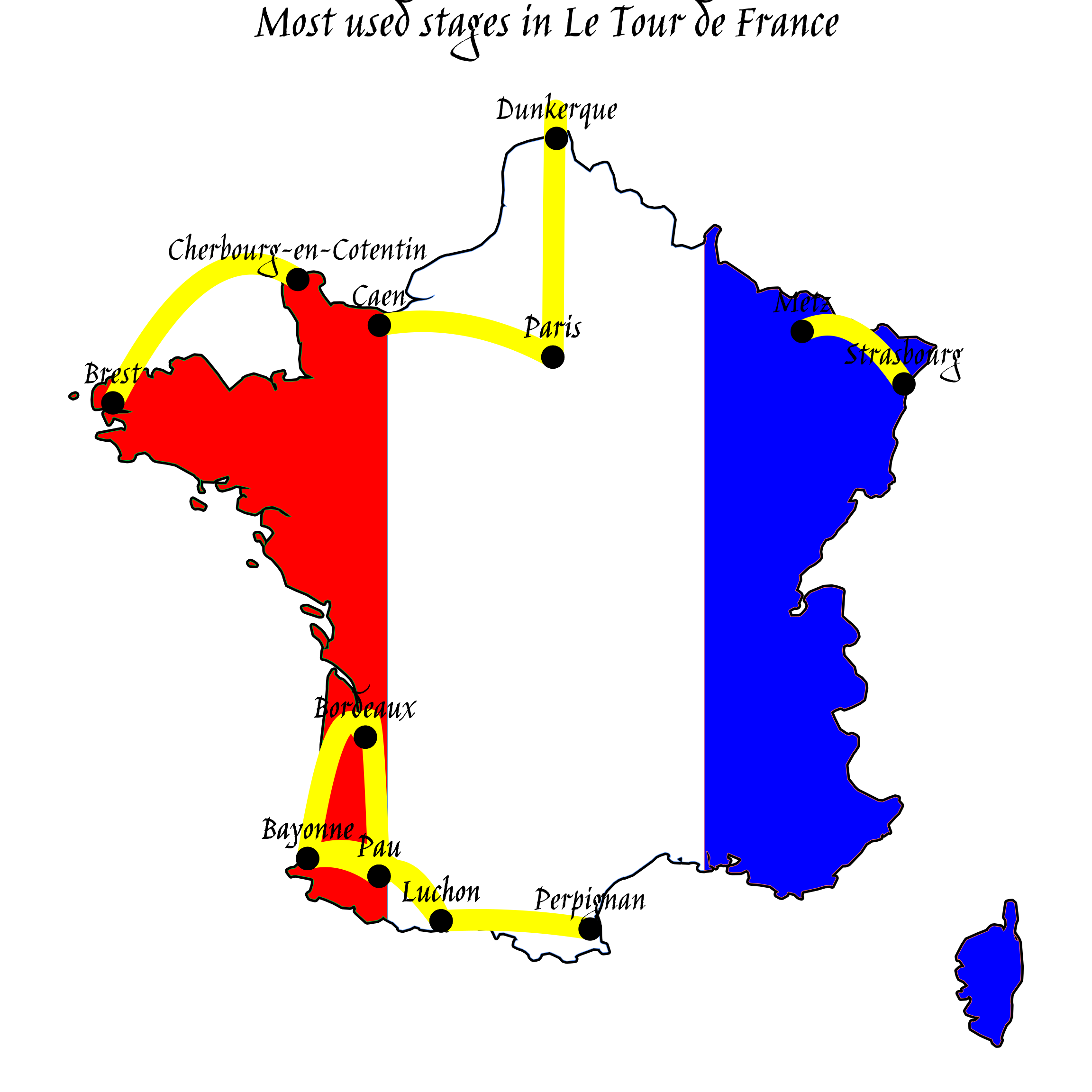

# Finally, render a table showing the top 10 routes
r <- top_routes_sf[,c("label", "count")] 
r <- st_drop_geometry(r)
names(r) <- c("Stage", "Occurrences")
knitr::kable(r, format="markdown")

Stage	Occurrences
Pau - Bordeaux	18
Luchon - Perpignan	17
Caen - Paris	14
Pau - Luchon	14
Strasbourg - Metz	13
Bayonne - Luchon	12
Bordeaux - Bayonne	12
Bayonne - Pau	10
Cherbourg-en-Cotentin - Brest	10
Dunkerque - Paris	10

18. Le Tour de France

The Map

Credits